I’ve made a load of models of small living particles being moved around in hydrodynamic models (have a look at a few of the posts here). Mostly larvae, but also seeds and other propagules. These things can swim, and they can change their buoyancy. They can alter their trajectories in water models, because the water moves at different speeds in different depths. So a slow swimming speed, when directed vertically, can have a dramatic impact on where they end up. Many larvae swim up and down in synchronicity with the tide from where they emerged. job’s done!

Well no. I got progressively uneasy with the end point of these models. One has to stop the model at some point and report where the particle ended up. But imagine the model stopping with a larvae, only a few mm’s in diameter, being swept along in tidal currents at 3 knots, 20 metres above a sand bank; how can you say that it stopped on that bank? Even if it could somehow sense that this was the place for it, how could it get out of the water column in time to land on that bank? It could be swept kilometres before it could swim down. So how do they do it?

It turns out, for oyster at least, that we have meticulous scientific evidence for how they get out of the water column and onto the places they are looking for. This was research done in 1975 (Cragg and Gruffydd 1975), where, as it happens, the authors had a completely different speculative explanation for the behaviour they recorded. What they recorded was that oyster larvae swim around for a while and then drop out of the water column, subsequently, they respond to very slight increases in pressure by swimming up again. In tidal areas; when the water gets deeper – the tide is coming in, so a larva that swam upward on that cue would be swept inshore (on average, in general, etc. etc.).

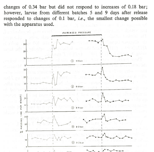
Here above is a screen capture from that paper in 1975. It shows how oyster larvae in the lab swim up from the bed at a selection of pressures from 0.1 Bar to 1 Bar (dependent on age (time in the water column)). 0.1 Bar would represent 1 m of incoming tide. A key aspect of this, for me, is the use of the bed as a reference pressure; from the bed the larvae can reliably sense very small changes in pressure – thus respond to tides. If they are in the water column without a reference it would be very difficult for them to tell if a slight pressure change was due water currents pushing them vertically, or tide, or atmospheric pressure changes.

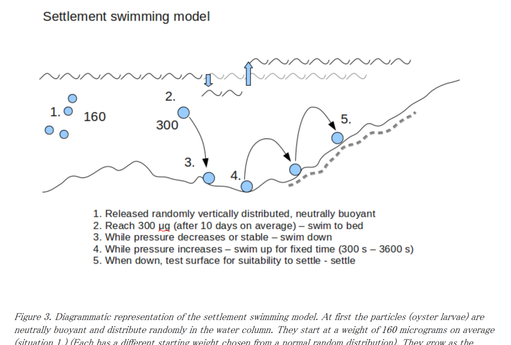
So a simple model of settlement comes to mind. Let all the larvae in the model drop out of the water column after a certain amount of time being swept around in the currents. Then let them bounce up and down until they bounce down on a suitable substrate. There they can settle. Or not. Depending on the quality of the substrate. So we have to define the quality of the substrate all over the model. We could start with depth (not too deep and not too shallow), but we could look at areas of previous settlement, or substrate type (sand, mud, rock etc.). Either way we end up with a settlement surface over the area of the model which represents how likely it is for a larvae to settle at any point. This can easily be defined as a probability surface – where the likelihood of settlement is defined for each grid square in a grid of squares laid over the model. So if the settlement probability is say 50% in a particular grid cell, and say 300 larvae bounce down on that cell -150 of them will settle and stay there. The others will bounce off and continue in the model.

This model has some immediate additional benefits: 1) The known good areas for settlement can be quite extensive and this model would show a pattern of settlement within the known area. 2) The larvae would be bouncing around in places where they may never settle and so disturbance to some areas (through dredging or contamination etc.) may have impacts on settlement patterns even though the settlement areas themselves remained undisturbed – the model may show this as the model tracks the journey as well as the end point.

Anyhow, we made the model and wrote the paper and you can read it if you’d like (just Google “willis oysters solent” or somesuch or look at the ‘Scientific Publications’ section of this web site, or follow: this link). There were some really interesting results. But it’s only a model. So these surprising results are just ideas that may be used in the process of hypothesis creation. Hypotheses which can be falsified through designed experiments or new observations. Thus the process of discovery advances through the scientific method. Here’s some interesting results:

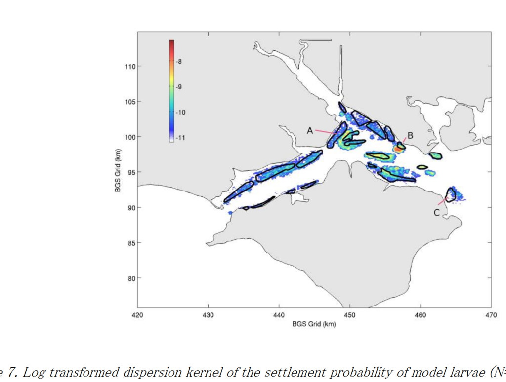
Here’s the pattern of settlement produced by the model. It was very different from the pattern expected by looking at the settlement surface. In particular the very high numbers settling on Browndown Bank (B on the figure above). This is a major hotspot in the Solent. It is a very interesting place to sail by. Take a look next time you are in the area. It is unique. 

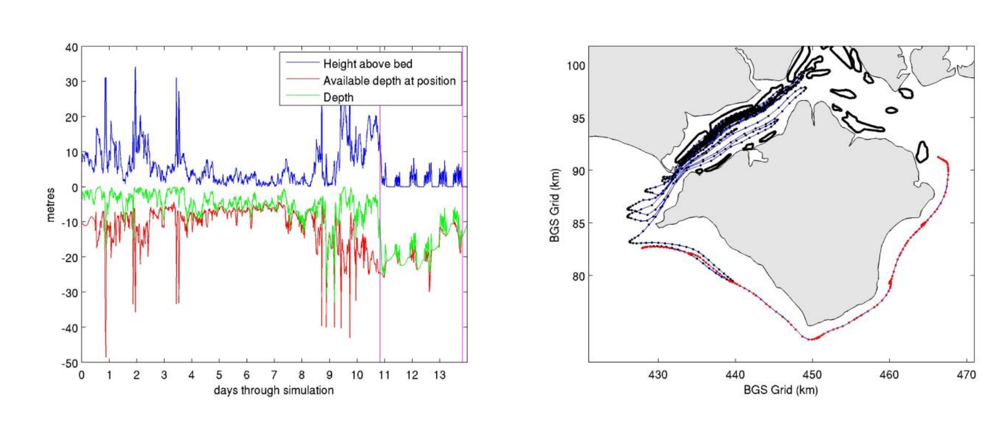
The above figure shows a single journey made by a model larvae. We ran the model for 10’s of thousands of larvae. Here the journey before and after settlement can be seen in both of two different views. On the left is a representation in numbers. The red line shows the total depth at each point in the journey, and just before 11 on the x-axis the purple vertical line indicates when the larva hit the bed and subsequently entered the bounce phase of its journey. There are 5 and a half periods of bouncing (through 5 incoming tidal cycles) and during this time the larvae manages to travel right round the south of the Isle of Wight. This can be seen as the red portion of the journey on the map panel of the right. It’s really interesting and unexpected, how the nature of the journey changes dramatically after the bounce settlement phase starts. It goes off in a completely different direction and stays well outside the entire area in which it was moving beforehand. This might show the total inadequacy of a model based only on the free swimming phase and suggests that the settlement model may be a very important addition to the swimming model.

The above video is one of the outputs made for the paper. It shows a batch of several thousand lavae leaving from the beds of known previous inhabitation and the results were used to measure modelled return and settlement.

What’s next? Why don’t we put some larvae down in a closed chamber and photograph their bounces? In effect recreate the experiments of 1975 in the field and see how the larvae actually react to the tidal cues.

Here’s the orginal figure from Cragg and Gruffydd 1975:

References

Cragg, S.M., Gruffydd, L.D. (1975) The swimming behaviour and the pressure responses of the veliconcha larvae of Ostrea edulis (L ). In: Barnes, H. ( e d . ) Proceedings of the Ninth European Marine Biology Symposium, Oban, Scotland, 1974 Aberdeen University Press, Aberdeen, p 43-57

Here’s a few additional ideas about the Solent. First using Lagrangian Coherent Structure analysis. This is a way of looking for structure in the ocean caused by water movements, so things like areas of downwelling or upwelling. Basically the technique looks for areas of convergenece or divergence in the surface flow field. These represent areas where water is being pushed up or down.

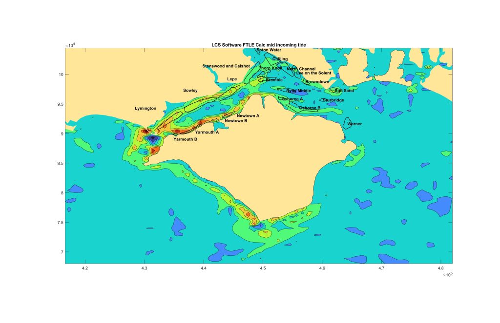
This is the FSLE (finite-size Lyapunov exponent ! ) situation at the mid flood tide mid spring neap cycle. So here the tide is flooding in, predominantly from the west.

All this is explained in the paper…Tew Kai, E., Rossi, V., Sudre, J., Weimerskirch, H., Lopez, C., Hernandez-Garcia, E., Marsac, F. and Garçon, V., 2009. Top marine predators track Lagrangian coherent structures. Proceedings of the National Academy of Sciences, 106(20), pp.8245-8250.

Trouble is that this doesn’t help very much and shows a mixed picture. I’ve seen seabirds massing over Browndown bank in the mid north east of the Solent, but the FSLE situation is low here, whereas it is much higher in the west. 

Another view is of bed shear stress (or average current velocity over the area (not exactly but closely related)…

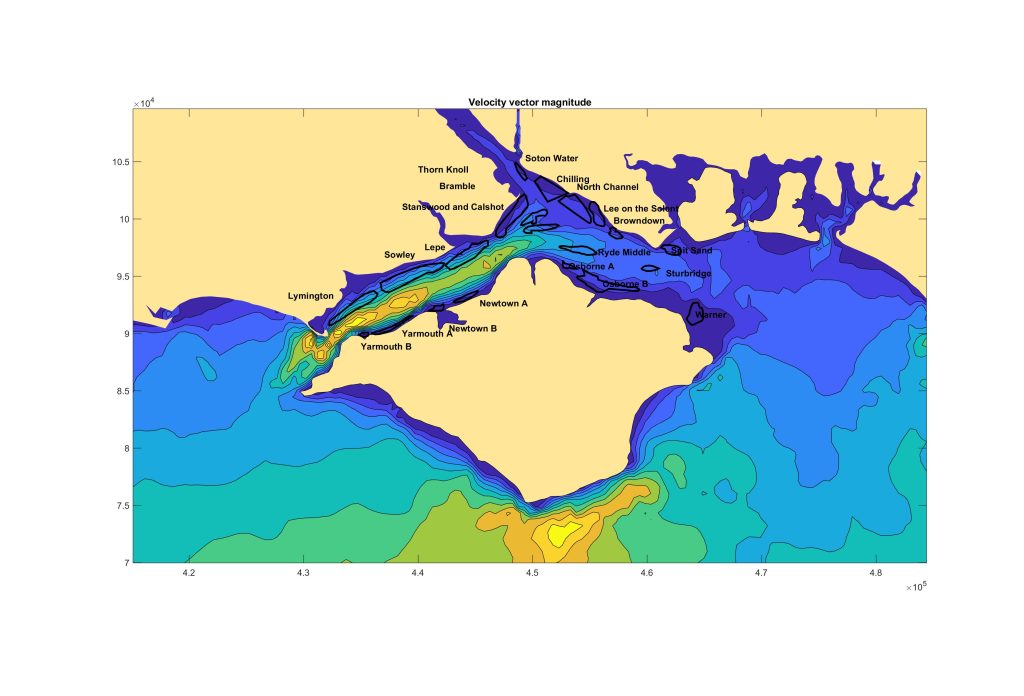
Again, interesting, but doesn’t help much.